
Software
Two Windows applications cover the recording and analysis of an eye-tracking study. Synocular calibrates each participant and records the session; Synocular Analysis turns the recordings into areas of interest, gaze maps, metrics and reports. Both come with the tracker.
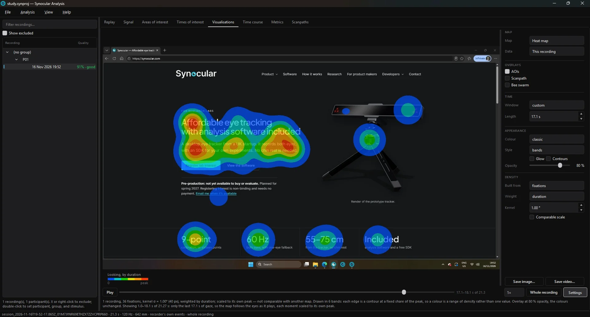
Screenshot of Synocular Analysis.

Synocular
Setup, calibration, validation, live gaze and recording. Included in the Windows installer.

Synocular Analysis
Areas of interest, gaze maps, metrics, time courses and reports, for one recording or a whole study.
Calibrate and record
Set up the tracker, calibrate each participant and record gaze. It finds both eyes and computes gaze 60 times a second.
The session file is a documented, versioned format with a Python reader, and synocular-export converts it to BIDS, EyeLink ASC or Tobii TSV.
From recordings to results
It opens a study, with its recordings, participants, groups and stimuli, and analyses it in place. Areas of interest and bookmarks are saved beside each recording, which stays exactly as it was made.
Replay
Play a recording back over its screen capture, with the gaze point, its trail, and fixations, saccades and blinks on a timeline. Bookmark a moment to come back to, or export the replay as a video.
The signal
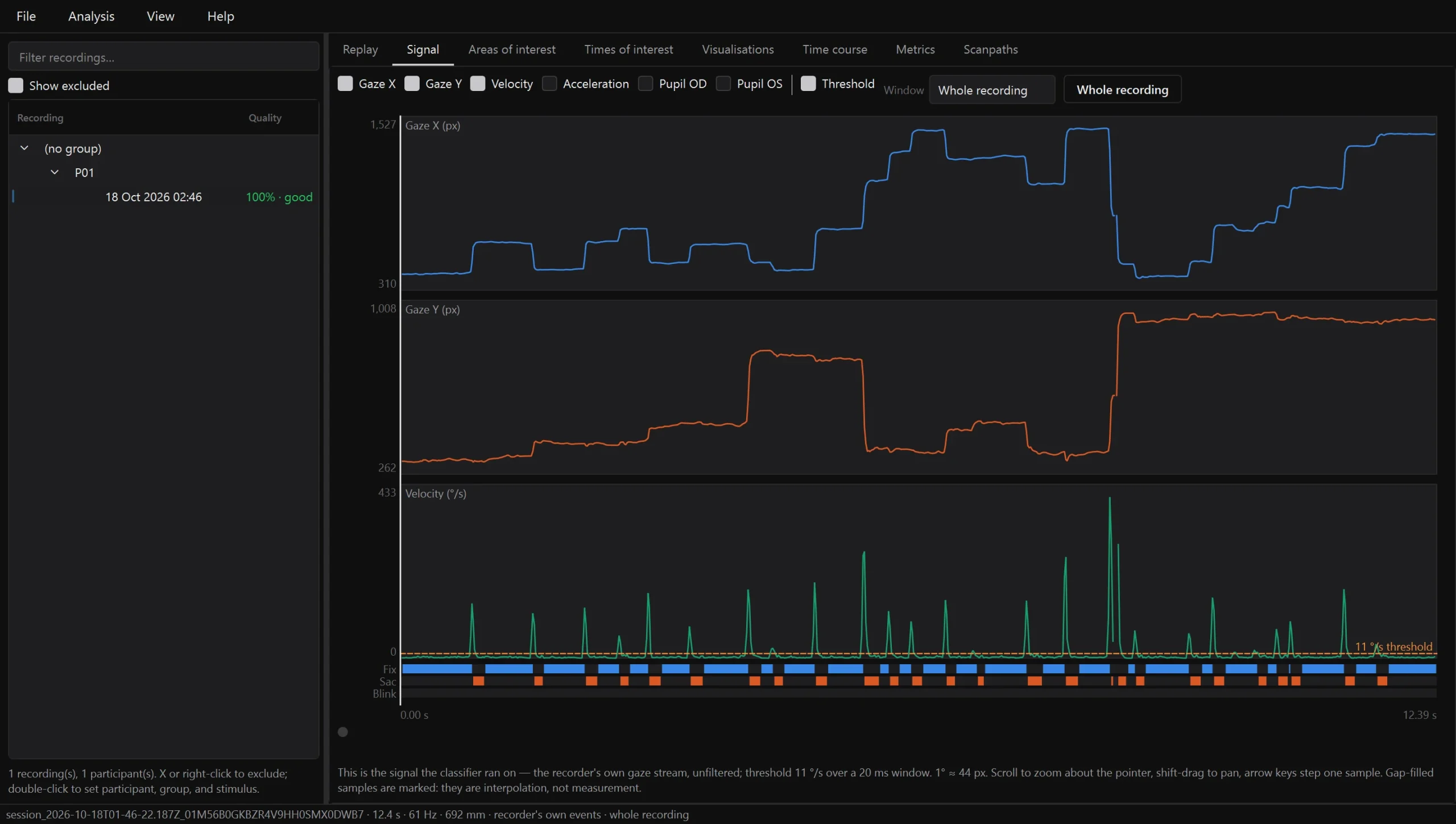
Gaze, velocity, acceleration and pupil size on one time axis, with the classified events underneath and the velocity threshold drawn on the axis it applies to. It is the exact signal the classifier ran on, so a threshold cutting in the wrong place shows on screen.
Events come from the recorder, or are detected again offline with I-VT or I-DT. Every threshold is reported with its unit, ready to quote.
Areas of interest
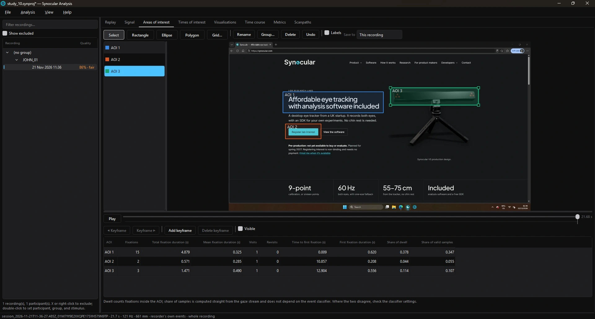
Rectangles, ellipses, polygons and grids, drawn on the stimulus or the screen capture. Keyframed areas follow content that moves. Each area shows its statistics as it is drawn.
Times of interest split a recording into windows (fixed, repeating, or built from bookmarks), and every table and chart is then reported per window.
Gaze maps
Heat, focus, gap and cluster maps over a stimulus image or the recording’s own screen capture, with the gaze plot, AOI outlines and the bee swarm as overlays on any of them. The bee swarm draws every gaze sample as a dot, the left and right eye in their own colours.
A heat map is drawn smooth, vivid or in flat bands, with or without outlines, in eight colour schemes and at any opacity. In every style one colour stands for one density, so the map reads against its key.
Drag the playhead to see what had been looked at by that moment, or press Play to watch the map build, as here. A trailing window plays the map as a moving view instead. Difference maps subtract one group’s attention from another’s, on a scale centred on zero.
Time course
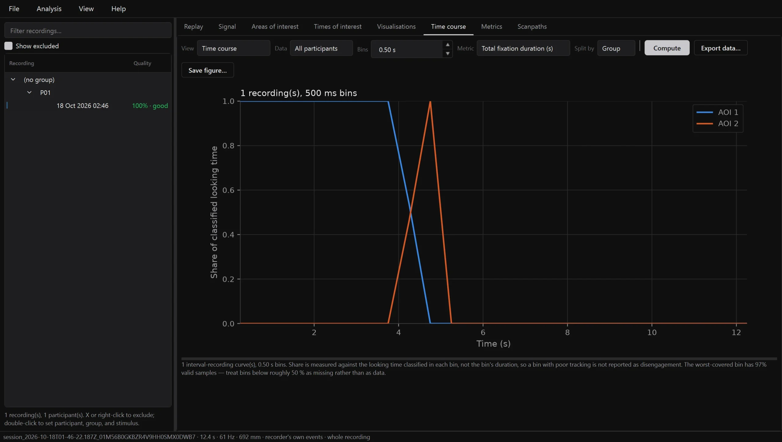
The share of looking on each area of interest, bin by bin, averaged across participants with a standard-error band. It exports in the long form that growth-curve and cluster-permutation analyses expect.
Scanpaths from different participants are compared by edit distance, ScanMatch and MultiMatch.
Measures, split by group
Tables split by group or by any participant variable, with effect sizes and tests. Fixation counts and dwell times for an area nobody looked at are zero; measures that do not exist for it, such as time to first fixation, are left empty rather than set to zero. Each summary reports how many values it used.
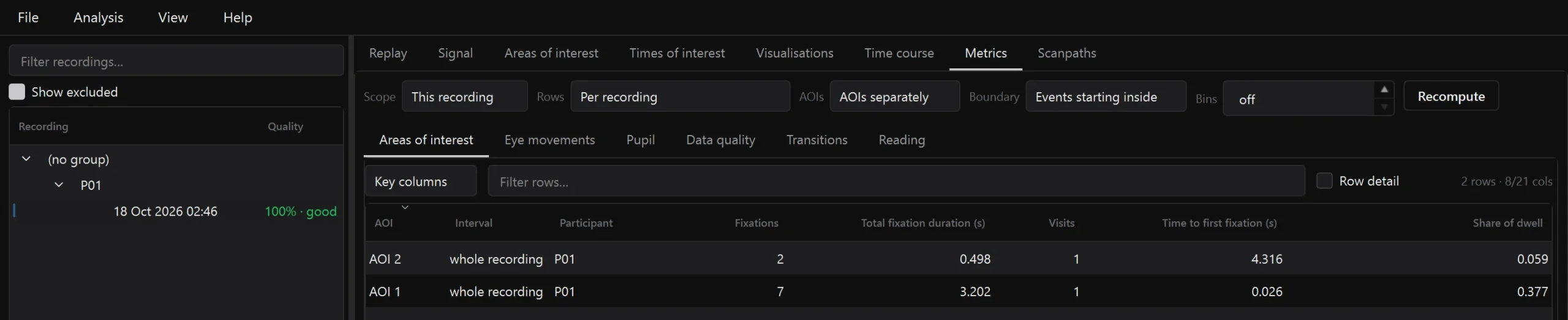
Methods you can report
Analysis › Analysis settings writes out every choice behind the numbers on screen: the recordings included, how events were classified, the time windows, the areas of interest and the screen geometry. Copy it into the methods section of a paper.
Reports are self-contained HTML pages for a session or a whole study, with the same methods and provenance section. Tables export as CSV, TSV or Excel, per sample, per event or per area.
Study: study-1
Events: as derived live by the recorder during the session; no offline re-classification.
Times of interest: none; each recording analysed whole, excluding its calibration sequence.
Boundary rule: events are assigned to an interval by onset.
Areas of interest: 2 region(s), from this recording’s sidecar.
Geometry: 1920×1080 px, viewing distance 692 mm, 1° ≈ 44 px.
Part of the text Synocular Analysis wrote for the recording above.
Desktop, command line or Python
The same engine runs the desktop application, a command-line tool that re-runs a whole study end to end, and a Python library for notebooks.
Software at a glance
| Software | What it does |
|---|---|
| Synocular | Setup, calibration, validation, live gaze and recording; the Windows installer |
| Synocular Analysis | Areas of interest, gaze maps, metrics, time courses and reports |
| synocular-export | Session files to BIDS, EyeLink ASC or Tobii TSV |
| SDKs and examples | Python client and C# examples; free to use with a Synocular tracker |
Synocular is supplied on a business-to-business basis, for research and development use. See Intended use & safety.